Two-dimensional segmentation fusion tool: an extensible, free-to-use, user-friendly tool for combining different bidimensional segmentations

1 Introduction

Contouring refers to the outlining of specific structures or areas in a target image. It entails defining the border of the foreground region (i.e., object of interest) and highlighting this border as a closed line of 1-pixel size in a 2D binary mask (i.e., black and white images). On the other hand, segmentation involves the definition of the foreground followed by the highlighting of this region with a dense surface, allowing the precise identification of a group of specific pixels (Hemalatha et al., 2018). This is a common image preprocessing step in several fields, ranging from autonomous driving, where vehicles, pedestrians, and road markings are segmented for detection and tracking purposes (Xiao et al., 2023), to agriculture/geology, where it is used to identify and classify different crops (Shoaib et al., 2022) or analyze soil conditions (Rippner et al., 2022). In the medical field, segmenting objects of interest is a widespread step, particularly in several fields of oncology (Jiménez and Racoceanu, 2019). For instance, in the context of radiotherapy, this involves delineating tumor volumes or areas at risk of microscopic disease, as well as normal anatomical structures, such as organs at risk. The goal of segmenting is to accurately define these structures to guide the radiation treatment process and ensure optimal patient outcomes (Lin et al., 2020). Similarly, segmenting objects is a very popular task in histology where the target is different, typically a microscopy image, but the main goal is to always spatially define the pixels belonging to different tissue regions for proceeding with further analysis (Bocchini et al., 2023).

Segmenting a cancer area is a time-consuming and labor-intensive task. It requires significant effort from practitioners, mainly medical doctors and physicians involved in cancer treatment planning (Hu et al., 2012), spending every day several hours of their working time in segmenting images. Typically, they use manual annotation tools [e.g., ImageJ; ROI Manager (Schneider et al., 2012) and AnaSP (Piccinini, 2015)] and computer-aided design (CAD) systems [e.g., MITK (Tasnadi et al., 2020a) and QuPath (Bankhead et al., 2017)]. However, in general, there are inter- (i.e., differences between segmentations created by different practitioners, also known as reproducibility) and intra-rater reliability (i.e., differences between segmentations created by the same practitioner but at different times, also known as repeatability) issues (Piccinini et al., 2017), and defining the correct segmentation (i.e., ground truth) is challenging. Accordingly, several statistical metrics and computational procedures are typically involved to determine the border of the object/area of interest in the image (Ramesh et al., 2021). These range from threshold-based segmentation approaches (Bai and Zhou, 2023) to deep-learning ones (Piccinini et al., 2023), never excluding the manual segmentation, which is still the gold standard for several applications (Veta et al., 2013). However, more 2D segmentation masks (typically represented as binary masks of the same size of the input image, with the object of interest identified by a white region on a black background) are available because they are (a) obtained in different ways, (b) or by different practitioners, (c) or by the same practitioner but at different times. Figure 1 shows the example of segmentations obtained by two different annotators, analyzing a slide scanner histological image, a microscopy cancer spheroid image, a magnetic resonance slide, a textile photograph, and an agricultural picture. In these cases, fusion algorithms are typically used for “fusing” (i.e., a process for combining, averaging, and “computing the mean”) multiple 2D segmentations. Nevertheless, nowadays, there is no standard for this procedure, and different fusing solutions have been proposed in the literature (James and Dasarathy, 2014).

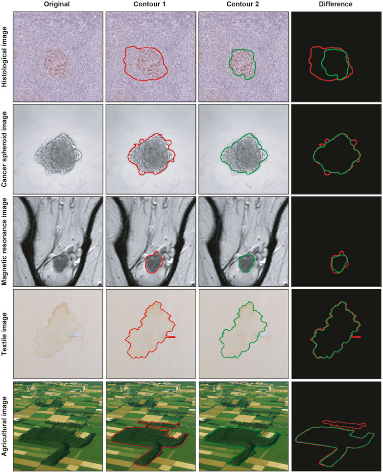
FIGURE 1. Example of segmentations obtained by two different practitioners. From top to bottom: histological image, cancer spheroid image, magnetic resonance image, textile image, and agricultural image. From left to right: original image, contour obtained from the first annotator, contour obtained from the second annotator, and overlaid contours.

In this work, in addition to reviewing all the fusion algorithms proposed in the literature for averaging different 2D segmentations, we developed the Two-Dimensional Segmentation Fusion Tool (TDSFT), an extensible, user-friendly MATLAB (i.e., Matrix Laboratory) tool collecting more fusion algorithms. Free-to-use standalone versions have been provided for MAC, Linux, and Windows, and the MATLAB source code can be openly read. A commercial license of MATLAB is needed just in case the user wants to modify the code. The TDSFT simply requires a series of 2D binary segmentations as input (i.e., binary masks of the same size of the input image, with the object of interest identified by a dense white region on a black background) and provides a new binary mask with a white one-size pixel closed line of the foreground’s contour as output, computed according to the fusion algorithm and closing method selected. Therefore, the TDSFT can support medical specialists, but it can also be used in other fields where it is required to combine 2D closed lines.

The current version of TDSFT (i.e., version 1) offers eight different fusion algorithms to average multiple 2D segmentations and four fitting/interpolating methods for closing eventually sparse 2D lines. In addition, the TDSFT is designed to be easily extended with new fusion algorithms thanks to a dedicated graphical user interface (GUI) for configuring new parameters. A TDSFT source code, free-to-use standalone applications for MAC, Linux, and Windows, video tutorial, documentation, and sample datasets are available at the following link: https://sourceforge.net/p/tdsft.

2 Methods

In the next sections, the TDSFT’s structure, the four available fitting/interpolating methods, and the eight implemented fusion algorithms are described in detail.

2.1 Two-dimensional segmentation fusion tool—Backbone

The TDSFT is an extensible, free-to-use, user-friendly tool that offers several algorithms for the fusion of multiple bidimensional segmentations (Figure 2A). The TDSFT is developed using MATLAB R2022b as a modular and organized structure project developed using the model-view-controller (MVC, Supplementary File 1) pattern, strongly helping for extension. Accordingly, in case of literature published on new reliable fusion algorithms, it will be easy to include them in the tool. To be able to use the software without a license, the TDSFT is also available as a standalone application for Windows, Linux, and MAC.

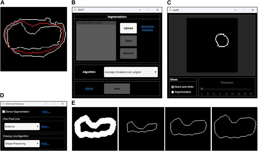
FIGURE 2. Fusion of 2D segmentations. (A) Example of bidimensional segmentation fusion using the algorithm named “Average Smallest and Largest.” (B) Main graphical user interface for loading and managing the 2D segmentations and selecting the fusion algorithm to be used. (C) Preview GUI for analyzing the single 2D segmentations. (D) Advanced feature GUI for optional parameters. (E) Examples of 1-pixel lines extracted by an original 2D segmentation larger than one pixel. From left to right: internal 1-pixel line, middle skeletonized 1-pixel line, and external 1-pixel line.

The TDSFT’s input is composed of a series of binary segmentations (several image formats are supported, including the classical tif, bmp, and png), which is managed through the main GUI with the “Upload,” “Open,” and “Remove” buttons (Figure 2B). In particular, the single-uploaded segmentations can be analyzed in a separate GUI that is automatically visualized by clicking the “Open” button (Figure 2C). The users can then choose the algorithm to be used for the fusion process from the drop-down menu named “Algorithm.” Using the “Advanced Features” link, it is also possible to open the advanced feature window (Figure 2D) for deciding (a) how to compute the one-pixel segmentations in case of original segmentations composed by a line with a diameter of more than one pixel (the possible solutions are an “internal,” “middle,” or “external” line, Figure 2E); (b) the algorithm to be used just for closing possibly unclosed 1-pixel size contour lines that can be obtained as output from several fusion algorithms (Figure 3).

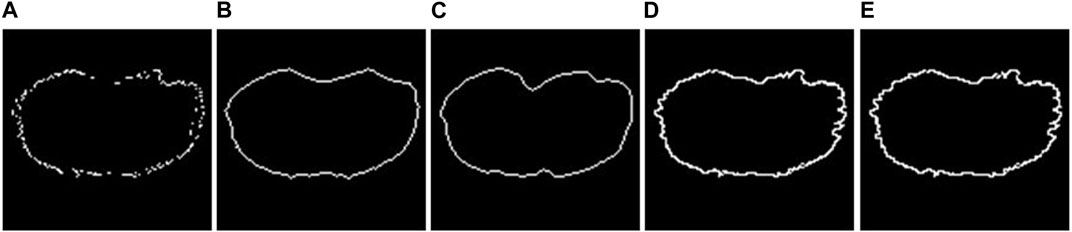
FIGURE 3. 2D fitting methods. (A) Example of an unclosed 2D segmentation. Example of results obtained using (B) Chan–Vese fitting method; (C) Geodesic Active Contour fitting method; (D) linear-based interpolation method; (E) shape-preserving-based interpolation method.

The closing methods offered can be divided into two groups: (I) Active contour methods: These methods iteratively adjust a contour’s position to align with object edges by minimizing an energy function that combines image and shape information. Not all the pixels of the original unclosed segmentation are preserved. (II) Interpolation methods: All the pixels of the original unclosed segmentation are preserved, and each pixel must be connected to at least two other points for obtaining a final closed line. The biggest issue, however, is to identify neighboring points for each pixel. In many circumstances, it can be difficult to find them in the Cartesian reference system. Because of this, the implementation option is to convert them to the polar reference point system and translate all coordinates around the largest segmentation’s center point. This enables them to order the points according to their angular position and use that information to identify their neighbors. Finally, a closed segmentation can be achieved by applying an interpolation method, creating a line between the pixels.

The algorithms belonging to the active contour group are implemented using built-in MATLAB functions as follows: (I1) Chan–Vese (Chan and Vese, 2001): It is designed to segment objects without clearly defined boundaries. This method relies on iteratively evolving sets of levels to minimize a multi-term function called energy. (I2) Geodesic (Caselles et al., 1997): It is based on active contours evolving in time according to intrinsic geometric measures of the image.

Instead, the interpolation methods are implemented by us, and they can also be found as external specific functions officially uploaded to the MathWorks file exchange website at the link: https://it.mathworks.com/matlabcentral/fileexchange/134951-closing-2d-line-with-interpolation. (II1) Linear interpolation: Each pair of adjacent points is connected by a segment that can be calculated independently of the others. If we denote (x_i, y_i) and (x_i+1, y_i+1) as the pair of adjacent points, the interpolating function f_i(x) is defined as reported in Eq. 1:

(II2) Piecewise cubic Hermite interpolation (PCHIP, shape-preserving) (Fritsch and Carlson, 1980): PCHIP interpolates using a piecewise cubic polynomial with these properties: (a) on each subinterval, the polynomial P(x) is a cubic Hermite interpolating polynomial for the given data points with specified derivatives at the interpolation points. (b) P(x) interpolates y, that is, P(x_j) = y_j, and the first derivative is continuous. The second derivative is probably not continuous, so jumps are possible. (c) The cubic interpolant P(x) is shape-preserving. The slopes at the x_j are chosen in such a way that P(x) preserves the shape of the data and respects monotonicity.

Furthermore, the TDSFT is extensible. Users can add and execute their fusion algorithms and closing methods. The process is supported by the documentation and the video tutorial. Furthermore, the user can set up a dedicated GUI for runtime parameters by just using a simple JSON file.

2.2 Implemented fusion algorithms—description

The TDSFT offers eight different fusion algorithms. In the next paragraphs, they are also described by exploiting the examples reported in Figure 4, showing the different algorithms’ output using the same input segmentation (Figure 4A). In addition, Supplementary File 2 reports flowcharts describing all their steps.

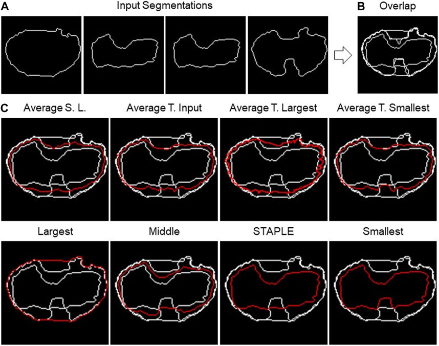
FIGURE 4. 2D fusion algorithms. (A) Example of four different input segmentations, one each panel and then (B) overlapped. (C) Example of results obtained using eight different fusion algorithms (the names are reported above the single panels) using the shape-preserving-based interpolation method when needed.

The first algorithm to be presented is named as “Largest,” which calculates the segmentation containing all the input segmentations. Basically, it is the contour of the “Union” of the different segmentations. The process consists of a few steps. As a first step, all segmentations are overlapped, then the hole-filling operation is performed, and finally, the perimeter of the resulting area is calculated.

The opposite algorithm to the previous one is called “Smallest,” which calculates the perimeter of the area shared by all segmentations. Essentially, it is the contour of the “Intersection” of the different segmentations. In this instance, the hole-filling procedure is carried out on all segmentations prior to completing the overlap. Then, appropriate matrices are then added to achieve their overlap. The area whose pixel value is equal to the number of segmentations is now referred to as the common area.

On the other hand, “Average Smallest And Largest” calculates the 1-pixel segmentation between the Smallest and the Largest segmentation. The Smallest and Largest segmentation are first calculated and are then overlapped. Finally, the skeletonization operation is applied to obtain the 1-pixel middle line.

The algorithms “Average Target Largest,” “Average Target Smallest,” and “Average Target From Input” are part of the same family of algorithms, with the only difference in the choice of target segmentation, the one from which the computation starts. In the first two, Largest and Smallest are used, and in the third, the user can choose the target between one of the input segmentations. After choosing the target segmentation, the process is the same for all these algorithms. Given a set of input segmentations and a target segmentation, the algorithm iterates over each pixel of the latter and for each of these computes the new pixel of the average segmentation. The process of obtaining a new pixel can be divided into two steps: (1) the closest pixel of any other segmentation to the chosen target segmentation’s pixel is calculated in order to create a group of points; (2) given the points obtained in step 1, the new pixel is calculated as follows: (a) if the points are two, the midpoint of the segment having these as extremes is calculated; (b) if the points are more than two but belong to the same line (collinear points), the two extremes are calculated, and the midpoint of the segment is calculated; (c) in other cases, the centroid of the polygon described by the set of points is calculated.

The next algorithm to be discussed is called “Middle,” which calculates the segmentation in the center of all the input ones. The first step is to overlap all the segmentations. Then, the algorithm operates in successive steps, and at each iteration, the smallest and the largest segmentation are removed. The total number of iterations is defined as the lower bound (i.e., floor integer) of (N.Seg. −1)/2, with N.Seg., and the number of available segmentations. At the end of the iterations, there are two possible situations: (1) if the number of input segmentations is odd, and then at the end of the iterations, only one segmentation will remain, which will then be the central segmentation; (2) if the number of input segmentations is even, on the other hand, there are two remaining segmentations. To obtain the result, the practitioner must specify the algorithm to be used to fuse the last two segmentations. The algorithms offered for this purpose are Average Smallest and Largest, Largest, and Smallest.

The last algorithm is “Simultaneous Truth and Performance Level Estimation (STAPLE)” (Warfield et al., 2004). STAPLE is a weighted voting algorithm that takes into account all segmentations while computing the outcome. As an initial step, the algorithm will combine all the segmentations into a test segmentation by simply voting on each pixel. STAPLE will rate each annotator’s accuracy in relation to this initial test segmentation. Then, it will redraw a new segmentation by weighting the votes of the specialists according to their accuracy. Because STAPLE is iterative, this cycle of estimating the accuracy and redrawing the test segmentation will repeat until the test segmentation stops changing or the maximum number of iterations is reached. The final test segmentation will be the “ground truth” that STAPLE returns. The implementation used in the TDSFT can be found at the following link: https://www.mathworks.com/matlabcentral/fileexchange/56789-staple-d.

3 Experiments

Comparing the different fusion algorithms and defining which is the best one is really challenging because there is not a general best one, and the better one depends on several factors (e.g., the presence of outlier segmentations and availability of many similar segmentations making the dataset unbalanced). This is the reason why we provided the user of several algorithms and not just a “winning” one. However, to provide a proof of concept on how the algorithms perform, we selected a representative case of study, a microscopy dataset that is publicly available, composed by different segmentations, obtained using freely available tools, and a manual ground truth. In the next sections, the experimental setup, the used metric, and the results obtained are described in detail.

3.1 Experimental setup—description

To analyze the performances of the different fusion algorithms, we used a dataset related to a cancer multicellular spheroid, imaged with a light-sheet fluorescence microscope (LSFM) (Stelzer et al., 2021). Tasnadi et al. (2020b) already used this dataset, testing several segmentation algorithms and disclosing all their specifics (which are not relevant to our research in this case). The spheroid is composed of 52 cells, and for each cell, the dataset includes two manual segmentations, one created by an expert microscopist operator and one created by a microscopist researcher, with a limited number of years of experience and five different segmentations automatically obtained using different freely available tools, precisely 3D-Cell-Annotator (3DCA) (Tasnadi et al., 2020b), MINS (Lou et al., 2014), Pagita (Gul-Mohammed et al., 2014), XPIWIT (Bartschat et al., 2016), and OpenSegSpim (Gole et al., 2016).

The images of the multicellular spheroid are 3D, precisely a 3D stack with each image representing a different z section of the spheroid. However, the TDSFT accepts as input binary two-dimensional (2D) segmentations. Accordingly, the procedure applied to create the testbed for the experiments are as follows: (a) 10 different sections from the 3D stack were randomly selected; (b) for each section, a cell was randomly chosen; (c) for each selected cell and selected section, the manual segmentation created by the expert microscopist was considered the ground truth, and the six other segmentations (i.e., second human annotator, 3DCA, MINS, Pagita, XPIWIT, and OpenSegSpim) were used for testing the different fusion algorithms. The configuration set for the advanced features was the default one, basically with the parameters “External one-pixel line” for pre-processing the input binary 2D segmentations, and “Shape-preserving” as the closing method in case of sparse pixels. Furthermore, specifically for the algorithm “Average Target From Input,” the target segmentation selected was the one obtained using 3DCA.

The dataset used in the experiments of this work is publicly available for further analysis at the following link: https://sourceforge.net/p/tdsft.

3.2 Performance metric—description

The most appropriate way to carry out the comparison of segmentations is so far unclear (Warfield et al., 2004). In the literature, several metrics have been proposed to compare segmentations. Simply measuring the volume of segmented structures (Iosifescu et al., 1997; Warfield et al., 2000) or assessing the limits of agreement (Bland and Altman, 2003) of volume estimates derived from the segmentations is something common. However, measures of spatial overlap are the metrics most widely applied (Dice, 1945). Alternative metrics have been sought (Everingham et al., 2002). For instance, in many applications, assessment of boundary differences is useful, and the Hausdorff measure and modifications have been used (Gerig et al., 2001). In addition, agreement measures, such as the kappa statistic, have also been explored (Zijdenbos et al., 1994). In conclusion, nowadays, there is not a single globally used metric for this purpose.

In our case, to compare the different fusion algorithms and evaluate the results obtained, we decided for the Jaccard index (JI), also known as Intersection over Union (IoU) or the Jaccard similarity coefficient (Piccinini et al., 2020). It is a well-known metric used for evaluating the similarity of two sample sets (e.g., A and B). JI (A and B) is mathematically defined as the size of the intersection (i.e., |A $\cap$ B|, the number of overlapping voxels) divided by the size of the union (i.e., |A $\cup$ B|) of the sample sets, according to Eq. 2:

3.3 Results

Table 1 reports the JI values obtained by analyzing the spheroid dataset (composed by the 10 different sections of the cells randomly selected, hereafter named Cell#, with # ranging from 1 to 10), and comparing with the ground truth the result of the different versions of the fusion algorithms. Precisely, the 10 different versions of the fusion algorithms compared are

1. Average Smallest And Largest.

2. Average Target From Input (3DCA), with the segmentation obtained using 3DCA as the target line.

3. Average Target Largest, with the segmentation obtained with the “Largest” algorithm used as the target line.

4. Average Target Smallest, with the segmentation obtained with the “Smallest” algorithm used as the target line.

5. Largest.

6. Middle—Average, with the final line computed using the “Average” algorithm in case of an even number of input segmentations.

7. Middle—Largest, with the final line computed using the “Largest” algorithm in case of an even number of input segmentations.

8. Middle—Smallest, with the final line computed using the “Smallest” algorithm in case of an even number of input segmentations.

9. Smallest.

10. STAPLE.

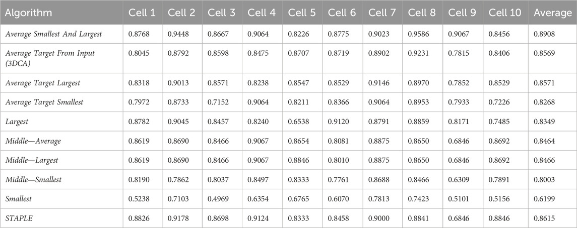
TABLE 1. Jaccard indexes of the fused segmentations obtained with the different algorithms.

Table 2 reports the rank’s position of the 10 different versions of the tested fusion algorithms, according to the average value of the JI (i.e., Table 1, last column) computed by considering together the 10 different cells. Despite the absolute values being dataset-dependent, it is possible to observe general results just by considering the rank positions of the fusion algorithms.

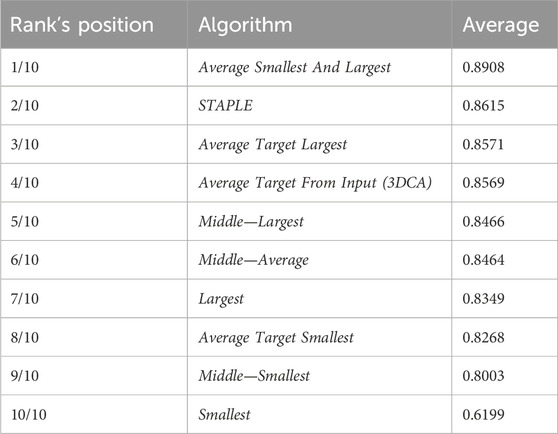
TABLE 2. Final rank’s positions of different fusion algorithms.

First of all, it is worth considering that in a set of data, the outer and the inner lines are most of the time noisy instances, called outliers. Translating this general concept to the segmentations, the Smallest and Largest algorithms, based on the definition of the outer and inner lines, are outlier-dependent and, in fact, are characterized by some of the worst performances (position 10/10 and 7/10 in the rank, respectively). All the algorithms based on the Average of the different segmentations (defined by considering a specific line as a target) obtained similar values, which were all reported in the central part of the ranking (rank’s positions 8/10, 4/10, and 3/10). Similarly, all the algorithms based on the selection as output of the line in the Middle obtained similar results with excellent absolute JI values, except for the algorithm Middle—Smallest (rank’s position 9/10) selecting the smallest line in the middle, in case of an even number of segmentations (like in this experiment where we used the fusion algorithms as input of six different segmentations). However, there is no reliable explanation for a so different result obtained by the Middle—Smallest (i.e., 9/10) algorithm in comparison to the Middle—Largest one (i.e., 5/10). Finally, the best results were obtained using STAPLE (rank’s position 2/10) and Average Smallest And Largest (rank’s position 1/10). However, STAPLE, considering the contribution of all the input segmentations, for minimizing the potentially large uncertainty on the values of the estimated parameters, is suggested in case of a high number of input segmentations to be fused (Commowick and Warfield, 2010), while Average Smallest And Largest, being based just on the outer and inner lines, is suggested in case of a limited number of segmentations to be fused. For instance, in the practical case of just two input segmentations (one of the most recurrent cases in real scenarios), Average Smallest And Largest would be preferred to STAPLE (absolutely not recommended in this scenario because it is not designed for working with just two segmentations). Nevertheless, Average Smallest And Largest, being based on the Largest and Smallest algorithms, is noise-sensitive. Accordingly, for filtering the outliers and being more robust, our general suggestion is the Middle—Average (i.e., 6/10) algorithm that selects the line in the middle, without interpolating in the case of an odd number of input segmentations and exploiting the Average algorithm in the case of an even number of inputs. In addition, it is worth noting that Average Smallest And Largest (i.e., 1/10), and Middle—Average (i.e., 6/10) give precisely the same output in the case of just two input segmentations.

4 Conclusion

Segmenting objects of interest, specifically the segmentation of tumor areas in medical images, is a crucial and challenging step in various fields, including oncology and histology. The accuracy of segmentation is pivotal in guiding further decisions, but the lack of a standard for identifying object boundaries introduces subjectivity and variability into the process.

The subjective nature of the segmentation is evident as different operators can produce varying segmentations for the same tumor image. Moreover, even the same operator may produce different segmentations when analyzing the same area at different times.

To solve the difficulty of fusing multiple 2D segmentations to determine a reliable foreground’s contour line, many algorithms have been developed. However, none of these algorithms has achieved validation or standardization, leaving an ongoing research gap in this field.

In this paper, we are interested in different fusion algorithms (not segmentation ones). In particular, this study introduces the TDSFT, a free-to-use, user-friendly tool developed to facilitate the fusion of multiple 2D segmentations. Precisely, we implemented different fusion algorithms and compared them using publicly available datasets composed by different segmentations previously obtained with segmentation tools already published and validated. It is worth noting that the TDSFT is not limited to medical applications but can be employed in any field requiring the combination of 2D closed lines. It provides an interface for users to choose from multiple fusion algorithms and offers flexibility for adding new algorithms through a graphical interface.

To evaluate the performance of the fusion algorithms, experiments were conducted using a dataset of multicellular spheroid images, JI as a similarity metric, and 10 different fusion algorithms. The Average Smallest And Largest and STAPLE algorithms showed promising results, with their suitability depending on factors like the number of input segmentations. However, the Middle—Average algorithm was the one finally suggested because it is a robust choice for filtering outliers and producing reliable fusion results.

In conclusion, this study contributes to the ongoing efforts to address the subjectivity and variability in object segmentation by describing various fusion algorithms and introducing the free-to-use, user-friendly TDSFT tool. As future work, exploiting the extensibility of the TDSFT, we would like to implement and test a new algorithm first by discarding the Largest and Smallest lines for removing probable outliers and then applying the Average Target From Input, by considering the line obtained by previously applying the Middle—Average algorithm as the target input. This combination would balance the values from all the input lines (except the outer and inner ones) and would be a good solution for filtering noise when there are at least three input segmentations. In addition, we would like to include an optimized procedure for a parallel analysis of multiple objects.

The TDSFT source code, standalone application for MAC, Linux, and Windows, video tutorial, documentation, and sample datasets can be downloaded from the following link: https://sourceforge.net/p/tdsft.

Data availability statement

The datasets presented in this study can be found in online repositories. The names of the repository/repositories and accession number(s) can be found at: https://sourceforge.net/p/tdsft.

Author contributions

FP: conceptualization, data curation, formal analysis, funding acquisition, investigation, methodology, project administration, resources, software, validation, visualization, and writing–original draft. LD: data curation, formal analysis, investigation, methodology, software, validation, visualization, and writing–original draft. J-CP: data curation, formal analysis, funding acquisition, investigation, resources, and writing–original draft. ML: data curation, formal analysis, investigation, validation, visualization, and writing–original draft. BKw: data curation, formal analysis, investigation, validation, visualization, and writing–original draft. BKu: data curation, methodology, resources, and writing–review and editing. AC: conceptualization, methodology, project administration, and writing–review and editing. GM: data curation, formal analysis, funding acquisition, resources, supervision, and writing–review and editing. GC: data curation, formal analysis, funding acquisition, resources, supervision, validation, and writing–review and editing.

Funding

The author(s) declare that financial support was received for the research, authorship, and/or publication of this article. FP, J-CP, ML, and GC acknowledge the support received from the MAECI Science and Technology Cooperation Italy–South Korea Grant Years 2023–2025 by the Italian Ministry of Foreign Affairs and International Cooperation (CUP project: J53C23000300003) and the National Research Foundation (Funding No.: 2022K1A3A1A25081295). All authors with IRCCS IRST affiliation acknowledge support by the Italian Ministry of Health, contribution “Ricerca Corrente” within the research line “Appropriateness, outcomes, drug value, and organizational models for the continuity of diagnostic therapeutic pathways in oncology”.

Acknowledgments

The authors thank Roberto Vespignani and Nicola Caroli (IRST, Meldola, Italy) for technical support; Mariachiara Stellato (Department of Physics and Astronomy “Augusto Righi,” Università di Bologna, Italy) for testing the tool; Massimo Passera (Science Counselor, Embassy of Italy, Seoul, South Korea) for important suggestions.

Conflict of interest

BK was employed by the Central R&D Center, Medical and Bio Decision (MBD) Co., Ltd.

The remaining authors declare that the research was conducted in the absence of any commercial or financial relationships that could be construed as a potential conflict of interest.

Publisher’s note

All claims expressed in this article are solely those of the authors and do not necessarily represent those of their affiliated organizations, or those of the publisher, the editors, and the reviewers. Any product that may be evaluated in this article, or claim that may be made by its manufacturer, is not guaranteed or endorsed by the publisher.

Supplementary material

The Supplementary Material for this article can be found online at: https://www.frontiersin.org/articles/10.3389/fbioe.2024.1339723/full#supplementary-material

Supplementary Data Sheet 1 | TDSFT MVC architecture.

Supplementary Data Sheet 2 | Flowcharts of the different algorithms.

References

Bai, R., and Zhou, M. (2023). SL-HarDNet: skin lesion segmentation with HarDNet. Front. Bioeng. Biotechnol. 10, 1028690. doi:10.3389/fbioe.2022.1028690
Bankhead, P., Loughrey, M. B., Fernández, J. A., Dombrowski, Y., McArt, D. G., Dunne, P. D., et al. (2017). QuPath: open source software for digital pathology image analysis. Sci. Rep. 7 (1), 16878–16887. doi:10.1038/s41598-017-17204-5
Bartschat, A., Hübner, E., Reischl, M., Mikut, R., and Stegmaier, J. (2016). XPIWIT—an XML pipeline wrapper for the Insight Toolkit. Bioinformatics 32 (2), 315–317. doi:10.1093/bioinformatics/btv559
Bland, J. M., and Altman, D. G. (2003). Applying the right statistics: analyses of measurement studies. Official J. Int. Soc. Ultrasound Obstetrics Gynecol. 22 (1), 85–93. doi:10.1002/uog.122
Bocchini, M., Tazzari, M., Ravaioli, S., Piccinini, F., Foca, F., Tebaldi, M., et al. (2023). Circulating hsa-miR-5096 predicts 18F-FDG PET/CT positivity and modulates somatostatin receptor 2 expression: a novel miR-based assay for pancreatic neuroendocrine tumors. Front. Oncol. 13, 1136331. doi:10.3389/fonc.2023.1136331
Caselles, V., Kimmel, R., and Sapiro, G. (1997). Geodesic active contours. Int. J. Comput. Vis. 22, 61–79. doi:10.1023/a:1007979827043
Chan, T. F., and Vese, L. A. (2001). Active contours without edges. IEEE Trans. image Process. 10 (2), 266–277. doi:10.1109/83.902291
Commowick, O., and Warfield, S. K. (2010). Estimation of inferential uncertainty in assessing expert segmentation performance from STAPLE. IEEE Trans. Med. imaging 29 (3), 771–780. doi:10.1109/TMI.2009.2036011
Dice, L. R. (1945). Measures of the amount of ecologic association between species. Ecology 26 (3), 297–302. doi:10.2307/1932409
Everingham, M., Muller, H., and Thomas, B. (2002). “Evaluating image segmentation algorithms using the pareto front,” in Computer Vision—ECCV 2002: 7th European Conference on Computer Vision, Copenhagen, Denmark, May, 2002, 34–48. doi:10.1007/3-540-47979-1_3
Fritsch, F. N., and Carlson, R. E. (1980). Monotone piecewise cubic interpolation. SIAM J. Numer. Analysis 17 (2), 238–246. doi:10.1137/0717021
Gerig, G., Jomier, M., and Chakos, M. (2001). “Valmet: a new validation tool for assessing and improving 3D object segmentation,” in Medical Image Computing and Computer-Assisted Intervention–MICCAI 2001: 4th International Conference, Utrecht, The Netherlands, October, 2001, 516–523. doi:10.1007/3-540-45468-3_62
Gole, L., Ong, K. H., Boudier, T., Yu, W., and Ahmed, S. (2016). OpenSegSPIM: a user-friendly segmentation tool for SPIM data. Bioinformatics 32 (13), 2075–2077. doi:10.1093/bioinformatics/btw093
Gul-Mohammed, J., Arganda-Carreras, I., Andrey, P., Galy, V., and Boudier, T. (2014). A generic classification-based method for segmentation of nuclei in 3D images of early embryos. BMC Bioinforma. 15 (1), 9–12. doi:10.1186/1471-2105-15-9
Hemalatha, R., Thamizhvani, T., Dhivya, A. J. A., Joseph, J. E., Babu, B., and Chandrasekaran, R. (2018). Active contour based segmentation techniques for medical image analysis. Med. Biol. Image Analysis 4 (17), 2. doi:10.5772/intechopen.74576
Hu, Y. C., Grossberg, M. D., Wu, A., Riaz, N., Perez, C., and Mageras, G. S. (2012). Interactive semiautomatic contour delineation using statistical conditional random fields framework. Med. Phys. 39 (7Part2), 4547–4558. doi:10.1118/1.4728979
Iosifescu, D. V., Shenton, M. E., Warfield, S. K., Kikinis, R., Dengler, J., Jolesz, F. A., et al. (1997). An automated registration algorithm for measuring MRI subcortical brain structures. Neuroimage 6 (1), 13–25. doi:10.1006/nimg.1997.0274
James, A. P., and Dasarathy, B. V. (2014). Medical image fusion: a survey of the state of the art. Inf. fusion 19, 4–19. doi:10.1016/j.inffus.2013.12.002
Jiménez, G., and Racoceanu, D. (2019). Deep learning for semantic segmentation vs. classification in computational pathology: application to mitosis analysis in breast cancer grading. Front. Bioeng. Biotechnol. 7, 145. doi:10.3389/fbioe.2019.00145
Lin, D., Lapen, K., Sherer, M. V., Kantor, J., Zhang, Z., Boyce, L. M., et al. (2020). A systematic review of contouring guidelines in radiation oncology: analysis of frequency, methodology, and delivery of consensus recommendations. Int. J. Radiat. Oncol. Biology* Physics* 107 (4), 827–835. doi:10.1016/j.ijrobp.2020.04.011
Lou, X., Kang, M., Xenopoulos, P., Munoz-Descalzo, S., and Hadjantonakis, A. K. (2014). A rapid and efficient 2D/3D nuclear segmentation method for analysis of early mouse embryo and stem cell image data. Stem Cell Rep. 2 (3), 382–397. doi:10.1016/j.stemcr.2014.01.010
Piccinini, F. (2015). AnaSP: a software suite for automatic image analysis of multicellular spheroids. Comput. Methods Programs Biomed. 119 (1), 43–52. doi:10.1016/j.cmpb.2015.02.006
Piccinini, F., Balassa, T., Carbonaro, A., Diosdi, A., Toth, T., Moshkov, N., et al. (2020). Software tools for 3D nuclei segmentation and quantitative analysis in multicellular aggregates. Comput. Struct. Biotechnol. J. 18, 1287–1300. doi:10.1016/j.csbj.2020.05.022
Piccinini, F., Peirsman, A., Stellato, M., Pyun, J. C., Castellani, G., Tazzari, M., et al. (2023). Deep learning-based tool for morphotypic analysis of 3d multicellular spheroids. J. Mech. Med. Biol. 23, 2340034. doi:10.1142/s0219519423400341
Piccinini, F., Tesei, A., Arienti, C., and Bevilacqua, A. (2017). Cell counting and viability assessment of 2D and 3D cell cultures: expected reliability of the trypan blue assay. Biol. Proced. online 19, 8–12. doi:10.1186/s12575-017-0056-3
Ramesh, K. K. D., Kumar, G. K., Swapna, K., Datta, D., and Rajest, S. S. (2021). A review of medical image segmentation algorithms. EAI Endorsed Trans. Pervasive Health Technol. 7 (27), e6. doi:10.3389/fbioe.2021.00006
Rippner, D. A., Raja, P. V., Earles, J. M., Momayyezi, M., Buchko, A., Duong, F. V., et al. (2022). A workflow for segmenting soil and plant X-ray computed tomography images with deep learning in Google’s Colaboratory. Front. Plant Sci. 13, 893140. doi:10.3389/fpls.2022.893140
Schneider, C. A., Rasband, W. S., and Eliceiri, K. W. (2012). NIH Image to ImageJ: 25 years of image analysis. Nat. methods 9 (7), 671–675. doi:10.1038/nmeth.2089
Shoaib, M., Hussain, T., Shah, B., Ullah, I., Shah, S. M., Ali, F., et al. (2022). Deep learning-based segmentation and classification of leaf images for detection of tomato plant disease. Front. Plant Sci. 13, 1031748. doi:10.3389/fpls.2022.1031748
Stelzer, E. H., Strobl, F., Chang, B. J., Preusser, F., Preibisch, S., McDole, K., et al. (2021). Light sheet fluorescence microscopy. Nat. Rev. Methods Prim. 1 (1), 73. doi:10.1038/s43586-021-00069-4
Tasnadi, E. A., Toth, T., Kovacs, M., Diosdi, A., Pampaloni, F., Molnar, J., et al. (2020a). 3D-Cell-Annotator: an open-source active surface tool for single-cell segmentation in 3D microscopy images. Bioinformatics 36 (9), 2948–2949. doi:10.1093/bioinformatics/btaa029
Tasnadi, E. A., Toth, T., Kovacs, M., Diosdi, A., Pampaloni, F., Molnar, J., et al. (2020b). 3D-Cell-Annotator: an open-source active surface tool for single-cell segmentation in 3D microscopy images. Bioinformatics 36 (9), 2948–2949. doi:10.1093/bioinformatics/btaa029
Veta, M., Van Diest, P. J., Kornegoor, R., Huisman, A., Viergever, M. A., and Pluim, J. P. (2013). Automatic nuclei segmentation in H&E stained breast cancer histopathology images. PloS one 8 (7), e70221. doi:10.1371/journal.pone.0070221
Warfield, S. K., Mulkern, R. V., Winalski, C. S., Jolesz, F. A., and Kikinis, R. (2000). An image processing strategy for the quantification and visualization of exercise-induced muscle MRI signal enhancement. J. Magnetic Reson. Imaging 11 (5), 525–531. doi:10.1002/(sici)1522-2586(200005)11:5<525::aid-jmri8>3.0.co;2-2
Warfield, S. K., Zou, K. H., and Wells, W. M. (2004). Simultaneous truth and performance level estimation (STAPLE): an algorithm for the validation of image segmentation. IEEE Trans. Med. imaging 23 (7), 903–921. doi:10.1109/tmi.2004.828354
Xiao, X., Zhao, Y., Zhang, F., Luo, B., Yu, L., Chen, B., et al. (2023). BASeg: boundary aware semantic segmentation for autonomous driving. Neural Netw. 157, 460–470. doi:10.1016/j.neunet.2022.10.034
Keywords: histology, oncology, microscopy, segmentation, image fusion, free-to-use tool, standalone application
Citation: Piccinini F, Drudi L, Pyun J-C, Lee M, Kwak B, Ku B, Carbonaro A, Martinelli G and Castellani G (2024) Two-dimensional segmentation fusion tool: an extensible, free-to-use, user-friendly tool for combining different bidimensional segmentations. Front. Bioeng. Biotechnol. 12:1339723. doi: 10.3389/fbioe.2024.1339723
Received: 16 November 2023; Accepted: 11 January 2024;
Published: 31 January 2024.
Edited by:
Ilaria Cacciotti, University Niccolò Cusano, ItalyReviewed by:
Clarence Yapp, Vector Test Systems, United StatesJakub Nalepa, Silesian University of Technology, Poland
Copyright © 2024 Piccinini, Drudi, Pyun, Lee, Kwak, Ku, Carbonaro, Martinelli and Castellani. This is an open-access article distributed under the terms of the Creative Commons Attribution License (CC BY). The use, distribution or reproduction in other forums is permitted, provided the original author(s) and the copyright owner(s) are credited and that the original publication in this journal is cited, in accordance with accepted academic practice. No use, distribution or reproduction is permitted which does not comply with these terms.
*Correspondence: Filippo Piccinini, f.piccinini@unibo.it, filippo.piccinini@irst.emr.it